Distribution of values¶

The possible values of a variable, and how often they occur, is known as a distribution. It describes the likelihood of a particular value being observed. The distribution of step function values can be analysed in several different ways using staircase. The first thing to note is though is where most observed data corresponds to a finite sample, that is n observations, a step function corresponds to an infinite number of observations. Consequently, we cannot tally a count of values observed, but we can perform a value sum (analogous to pandas.Series.value_counts():

In [1]: sf = sc.Stairs().layer([0,1,2], [3,6,7]).mask((4,5))

In [2]: sf.plot()
Out[2]: <AxesSubplot:>

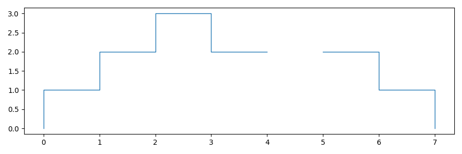
In [3]: sf.value_sums()
Out[3]: 
1.0    2
2.0    3
3.0    1
dtype: int64

The result of staircase.Stairs.value_sums() is a pandas.Series() where the index contains the observed values of the step function, and the values are the combined lengths of the intervals in the step function with that value. By default, the intervals where the step functions is undefined are omitted however this behaviour can be changed with the drop_na parameter:

In [4]: sf.value_sums(dropna=False)
Out[4]: 
1.0    2
2.0    3
3.0    1
NaN    1
dtype: int64

Consider this example of a step function with datetime domain:

In [5]: df = sc.make_test_data(dates=True, positive_only=True, seed=42)

In [6]: sf = sc.Stairs(df, "start", "end")

In [7]: sf.plot();

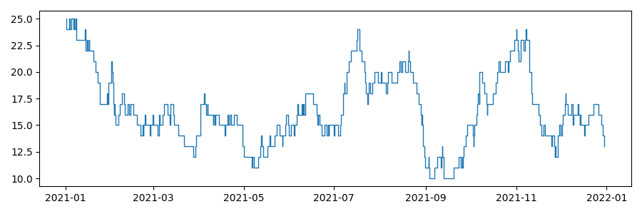
When the domain of a step function is datetime based then the result will be expressed as pandas.Timedelta.

In [8]: sf.value_sums()
Out[8]: 
  9 days 18:03:00
 13 days 05:28:00
 20 days 00:24:00
 18 days 00:35:00
 36 days 05:29:00
 61 days 14:49:00
 47 days 17:09:00
 40 days 07:02:00
 20 days 03:39:00
 20 days 09:55:00
 23 days 11:01:00
 14 days 21:52:00
 15 days 06:09:00
 13 days 01:03:00
  5 days 23:30:00
  3 days 00:50:00
dtype: timedelta64[ns]

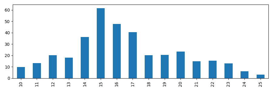
Conversion from pandas.Timedelta to a numerical representation can be done by dividing the result by a unit timedelta. The following example demonstrates how to convert the values to days and plot the distribution with pandas’ bar plot.

In [9]: hist_days = sf.value_sums()/pd.Timedelta(1, "day")

In [10]: hist_days
Out[10]: 
   9.752083
  13.227778
  20.016667
  18.024306
  36.228472
  61.617361
  47.714583
  40.293056
  20.152083
  20.413194
  23.459028
  14.911111
  15.256250
  13.043750
   5.979167
   3.034722
dtype: float64

In [11]: hist_days.plot.bar();

Histograms¶

To combine the observed values into bins we could group the index values of the Series and sum them, however an alternative exists in the form of staircase.Stairs.hist(). This method has a bins parameter, similar to that of pandas.Series.hist(). The bins parameter allows us to define the intervals with which to bin the observed values. For example, to create bins of width 2.

In [12]: sf.hist(bins=range(10, 27, 2))
Out[12]: 
[10, 12)             22 days 23:31:00
[12, 14)             38 days 00:59:00
[14, 16)             97 days 20:18:00
[16, 18)   88 days 00:11:00.000000003
[18, 20)   40 days 13:33:59.999999999
[20, 22)   38 days 08:52:59.999999998
[22, 24)   28 days 07:11:59.999999998
[24, 26)    9 days 00:19:59.999999999
dtype: timedelta64[ns]

In addition to defining bins, the method also permits the statistic to be defined for computing the value of each bin, via the stat parameter. The possibilities, inspired by seaborn.histplot() include

sum the magnitude of observations
frequency values of the histogram are divided by the corresponding bin width
density normalises values of the histogram so that the area is 1
probability normalises values so that the histogram values sum to 1

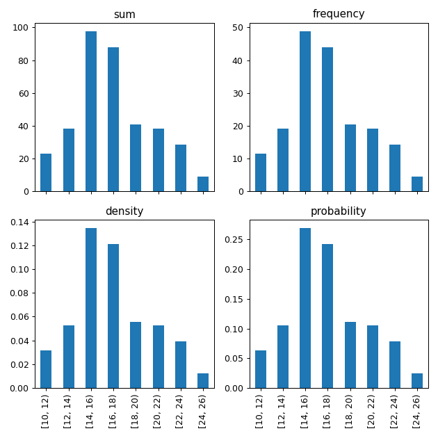
Histograms bar charts are one way of visualising a distribution, however they do have their drawbacks. Histograms can suffer from binning bias where the shape of the plot, and the story it tells, changes depending on the bin definition. An arguably better choice for visualising distributions is with the cumulative distribution function.

Cumulative distribution functions¶

This cumulative distribution function - perhaps better known as the ECDF, where the “E” standing for Empirical, signifying that the result is derived from observed data - describes the fraction of the distribution below each unique value in the dataset. It has several advantages over histogram plots for visualisation. This style of plot has been implemented in seaborn (seaborn.ecdfplot()) but can also be plotted with staircase too. In fact, the ECDF itself is a step function and its implementation in staircase is a derivation of the staircase.Stairs class, and is such inherits many useful methods such as staircase.Stairs.plot() and staircase.Stairs.sample().

In [13]: sf.ecdf
Out[13]: <staircase.ECDF, id=140343321848032>

In [14]: sf.ecdf.plot()
Out[14]: <AxesSubplot:>

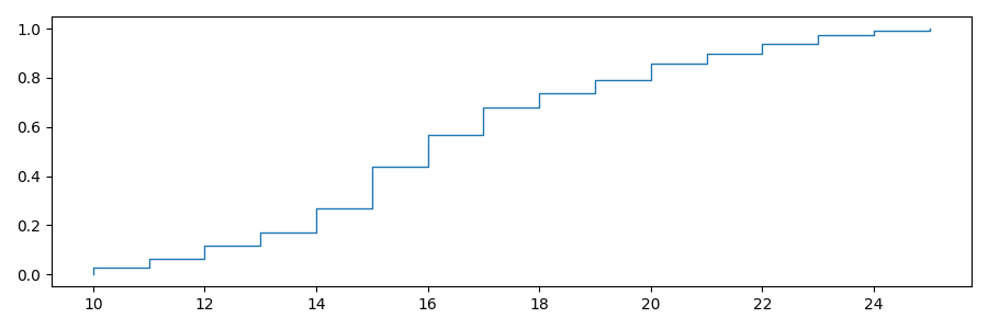
In [15]: print(f"{sf.ecdf(16) :.0%} of the time sf <= 16")
57% of the time sf <= 16

In [16]: print(f"{sf.ecdf(20) :.0%} of the time sf <= 20")
86% of the time sf <= 20

In [17]: print(f"{sf.ecdf(20) - sf.ecdf(16):.0%} of the time 16 < sf <= 20")
29% of the time 16 < sf <= 20

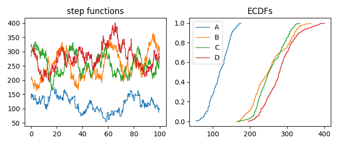
One of the strongest arguments for ECDFs over histogram plots is when several distributions are compared on the same plot.

In [18]: df = sc.make_test_data(dates=False, groups=["A","B","C","D"], seed=60)

In [19]: series = df.groupby("group").apply(sc.Stairs, "start", "end", "value")

In [20]: fig, axes = plt.subplots(ncols=2, figsize=(7,3))

In [21]: for i, stairs in series.items():
   ....:     stairs.plot(axes[0], label=i)
   ....: 

In [22]: axes[0].set_title("step functions");

In [23]: for i, stairs in series.items():
   ....:     stairs.ecdf.plot(axes[1], label=i)
   ....: 

In [24]: axes[1].legend();

In [25]: axes[1].set_title("ECDFs");

../_images/distribution_multiple_ecdf.png

Note that the ECDF is cached on each Stairs object so assigning it to a local variable will not improve efficiencies.

Fractiles, percentiles, quantiles¶

The ECDF is closely related to a couple of other functions, namely the fractile function and percentile function. The fractile function is the inverse of the ECDF:

In [26]: fig, axes = plt.subplots(ncols=2, figsize=(7,3))

In [27]: sf.ecdf.plot(axes[0]);

In [28]: axes[0].set_title("ECDF");

In [29]: sf.fractile.plot(axes[1]);

In [30]: axes[1].set_title("fractile function");

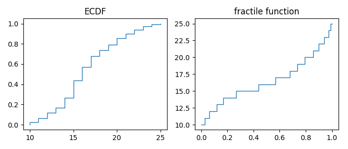
$../_images/distribution_ecdf_fractile.png$

The percentile function is identical in shape to the fractile function when plotting. This is because the two functions f(x) = p(x/100) where f and p are fractile and percentile functions respectively. Like the ECDF, the fractile and percentile functions are step functions and the corresponding implementations in staircase are classed derived from the staircase.Stairs class.

In [31]: print(f"The median value of the step function is {sf.fractile(0.5)}")
The median value of the step function is 16.0

In [32]: print(f"The 80th percentile of the step function values is {sf.percentile(80)}")
The 80th percentile of the step function values is 20.0

Choosing between fractiles and percentiles for a calculation is a matter of taste, but it is recommended to choose one, to avoid unnecessary calculation.

Closely related to the concept of fractiles, are quantiles, which are a set of cut points which divide a distribution into continuous intervals with equal probabilities. The cut points themselves are referred to as q-quantiles where q, an integer, is the number of resulting intervals. As a result there are q-1 of the q-quantiles, some of which may be already familiar:

The 2-quantile is more commonly known as the median.
The 4-quantiles (there are 3) are more commonly known as quartiles .
The 100-quantiles (there are 99) are more commonly known as percentiles.

Note, this definition of quantile differs from that used by pandas and numpy, whose implementation is equivalent to staircase.Stairs.fractile().

Slicing Array methods