Masking#
Prior to version 2, step functions in staircase had domains which were simply connected, meaning they were defined everywhere. The step function existed at every point between negative and positive infinity, with no gaps. This has changed in version 2, with step functions now able to have intervals where they are undefined. Areas where a step function is undefined are ignored when calculating statistics. For example, the following two step functions yield the same statistics - from mean, to variance, to percentiles.
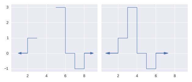
This feature is where masking finds is primary motivation. It allows us to perform a calculation over a subset of the step function’s domain. For example, using masking we can:
restrict a calculation to a particular interval, such as a year
exclude weekends from calculations
separate results by day of the week
There are three methods belonging to staircase.Stairs which allow us to perform masking: staircase.Stairs.clip(), staircase.Stairs.mask(), staircase.Stairs.where().
clip#
staircase.Stairs.clip() is not new in version 2. It retains the same method signature but its meaning has changed. In version 1 the clip function, given an interval in the domain defined by lower and upper parameters, would return a copy of the Stairs instance where the value of the step function outside of this interval is zero. In version 2 these values are undefined instead. That is, the clip method allows us to restrict the domain of a step function to an interval.
In [1]: sf = sc.Stairs(start=[2,3,4], end=[5,4,6], value=[1,2,-1])

In [2]: fig, axes = plt.subplots(ncols=2, figsize=(7,3), sharex=True, sharey=True)

In [3]: sf.plot(ax=axes[0], arrows=True);

In [4]: axes[0].set_title("sf");

In [5]: sf.clip(3,5).plot(ax=axes[1], arrows=True);

In [6]: axes[1].set_title("sf.clip(3,5)");
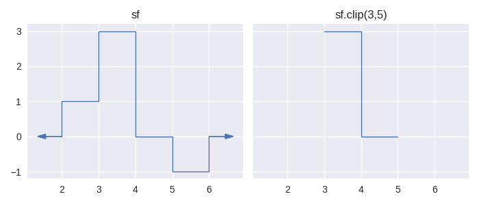
In version 1, there are several statistic methods which take lower and upper parameters to restrict a calculation to an interval. In version 2 these parameters have been removed in favour of using the method on a “clipped” step function, for example
In [7]: sf.clip(3,5).mean()
Out[7]: 1.5

In [8]: sf.clip(3,5).std()
Out[8]: 1.5

In [9]: sf.clip(3,5).min()
Out[9]: 0.0
Note that if there are multiple methods which will be applied to a clipped function, as is the case in the above example, then it is more efficient to assign the clipped Stairs instance:
In [10]: sf_clip = sf.clip(3,5)

In [11]: sf_clip.mean()
Out[11]: 1.5

In [12]: sf_clip.std()
Out[12]: 1.5

In [13]: sf_clip.min()
Out[13]: 0.0
On the topic of efficiency, the result achieved by staircase.Stairs.clip() can be achieved with both staircase.Stairs.mask() and staircase.Stairs.where() however these methods are more general and will not be as fast as clip.
mask/where#
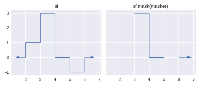
We introduce these methods together as they are two sides of the same coin, much like their counterparts in pandas, pandas.Series.mask() and pandas.Series.where(). These methods in pandas allow a user to set values in a Series to nan by supplying a boolean valued Series as a parameter. For pandas.Series.mask() it is the True values which yield nan and for pandas.Series.where() it is the False values *. The corresponding methods in staircase operate in much the same way, and utilise the concept of boolean values for step functions, as discussed in the tutorial on comparing step functions. For any two Stairs objects f and g:
the step function resulting from
f.mask(g)will be undefined wherever g is non-zero or undefinedthe step function resulting from
f.where(g)will be undefined wherever g is zero or undefined
Let’s see some examples:
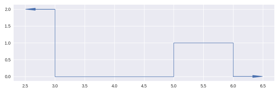
In [14]: masker = sc.Stairs().layer(None,3,2).layer(5,6);

In [15]: masker.plot(arrows=True)
Out[15]: <AxesSubplot: >
In [16]: fig, axes = plt.subplots(ncols=2, figsize=(7,3), sharey=True, sharex=True)

In [17]: sf.plot(ax=axes[0], arrows=True);

In [18]: axes[0].set_title("sf");

In [19]: sf.mask(masker).plot(ax=axes[1], arrows=True);

In [20]: axes[1].set_title("sf.mask(masker)");
In [21]: fig, axes = plt.subplots(ncols=2, figsize=(7,3), sharex=True, sharey=True)

In [22]: sf.plot(ax=axes[0], arrows=True);

In [23]: axes[0].set_title("sf");

In [24]: sf.where(masker).plot(ax=axes[1], arrows=True);

In [25]: axes[1].set_title("sf.where(masker)");
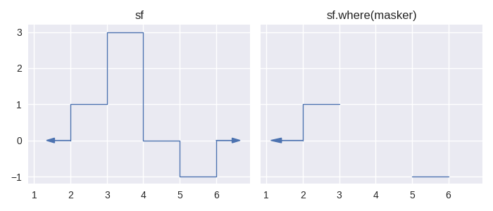
In particular, the staircase.Stairs.where() method, in combination with comparison operators can make for concise and readable calculations. For example, when calculating the integral for sf in the examples above, we arrive at a correct answer of 3. However the “area under the function” is given by 5. We can calculate this quantity like so:
In [26]: sf.where(sf > 0).integral() + (-sf).where(sf < 0).integral()
Out[26]: 5.0
Lastly, when using these two methods a tuple can be used as shorthand notation for simple step functions where (a,b) is equivalent to sc.Stairs(start=a, end=b). Using this convention .where((a,b)) gives an identical result to .clip(a,b), but as noted above using clip will be faster.
fillna#
As noted above, there are several methods that can be used for reducing the domain of a step function. Furthermore intervals not belonging to the domain are propagated through the application of arithmetic operators, logical operators and relational operators.
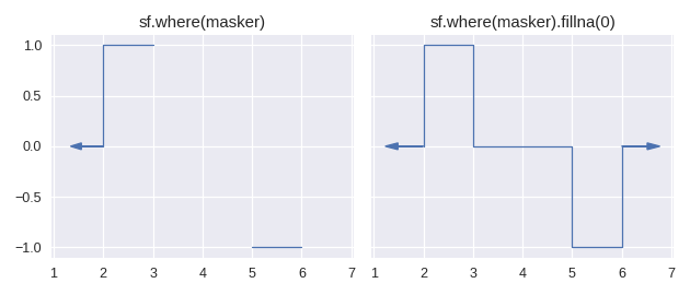
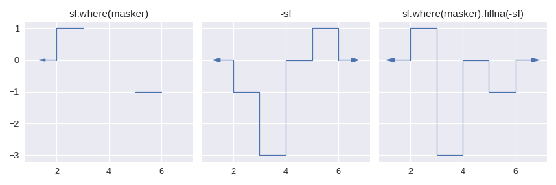
Currently there is only one method for enlarging the domain of a step function: staircase.Stairs.fillna(). This method is similar to its pandas counterpart pandas.Series.fillna(), in that it aims to replace null values, however it differs slightly in the semantics of parameters.
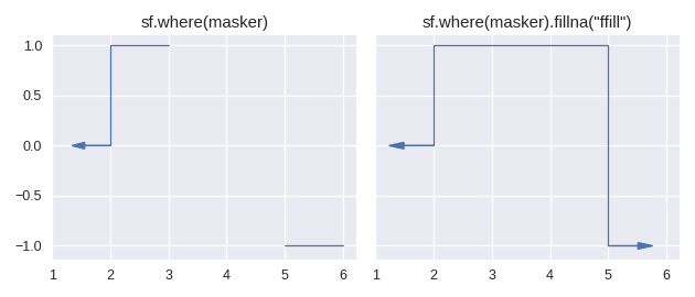
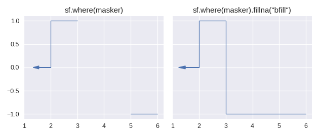
The method staircase.Stairs.fillna() takes one parameter, which can be either a real number, a staircase.Stairs instance, or a string corresponding to a method. These method names are taken from pandas and indicate the following behaviour:
pad / ffillpropagate last defined value forwardbackfill / bfillpropagate next defined value backward
For example:
isna/notna#
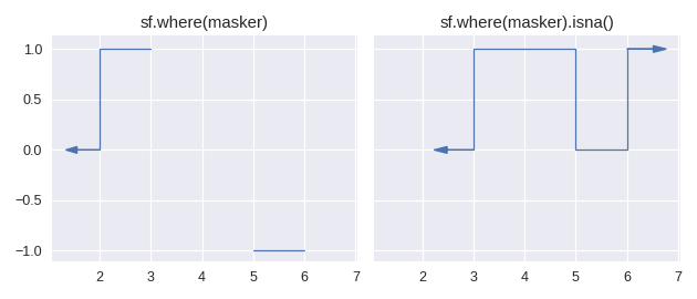
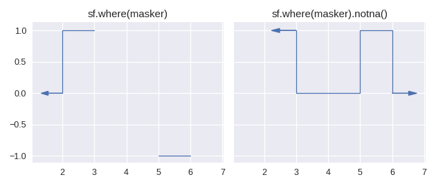
Finally, continuing on the theme of counterpart methods in pandas, we have staircase.Stairs.isna() and staircase.Stairs.notna() which return boolean valued step functions.
Footnotes
- *
Note that
pandas.Series.mask()andpandas.Series.where()are more general purpose than what is described here.